Chapter 4 LAGOS Analysis part 1

In this assignment, I used the R package ‘sf’ and other R packages to explore spatial operations in R markdown. I used data from LAGOS database to look at clean lake data in Minnesota, Illinois, and Iowa.

4.1 Loading in data

4.1.1 First download and then specifically grab the locus (or site lat longs)

# #Lagos download script
LAGOSNE::lagosne_get(dest_folder = LAGOSNE:::lagos_path())

## Warning in LAGOSNE::lagosne_get(dest_folder = LAGOSNE:::lagos_path()): LAGOSNE data for this version already exists on the local machine.
##   Re-download if neccessary using the 'overwrite` argument.'

#Load in lagos
lagos <- lagosne_load()

## Warning in (function (version = NULL, fpath = NA) : LAGOSNE version unspecified,
## loading version: 1.087.3

#Grab the lake centroid info
lake_centers <- lagos$locus

4.1.2 Convert to spatial data

#Look at the column names
#names(lake_centers)

#Look at the structure
#str(lake_centers)

#View the full dataset
#View(lake_centers %>% slice(1:100))

spatial_lakes <- st_as_sf(lake_centers,coords=c('nhd_long','nhd_lat'),
                          crs=4326) %>%
  st_transform(2163)

#Subset for plotting
subset_spatial <- spatial_lakes %>%
  slice(1:100) 

subset_baser <- spatial_lakes[1:100,]

#Dynamic mapviewer
mapview(subset_spatial)

4.1.3 Subset to only Minnesota

states <- us_states()

#Plot all the states to check if they loaded
#mapview(states)
minnesota <- states %>%
  filter(name == 'Minnesota') %>%
  st_transform(2163)

#Subset lakes based on spatial position
minnesota_lakes <- spatial_lakes[minnesota,]

#Plotting the first 1000 lakes
minnesota_lakes %>%
  arrange(-lake_area_ha) %>%
    slice(1:1000) %>%
  mapview(.,zcol = 'lake_area_ha')

4.2 Map outline of Iowa and Illinois (similar to Minnesota map upstream)

#creating Iowa map
iowa <- states %>%
  filter(name == 'Iowa')%>%
  st_transform(2163)

#creating Illinois map
illinois <- states %>%
  filter(name == 'Illinois')%>%
  st_transform(2163)

#combining Iowa and Illinois
il_ia <- rbind(iowa, illinois)

#mapping Iowa and Illinois
mapview(il_ia)

mapview code chunk is from https://r-spatial.github.io/mapview/articles/articles/mapview_02-advanced.html

4.3 Subsetting LAGOS data to these sites

#Subset iowa and illinois lakes based on spatial position 
il_ia_lakes <- spatial_lakes[il_ia,]

Combined, there are 16,466 lakes in Illinois and Iowa. Minnesota alone, has 29,038 lakes. This means that Minnesota has 12,572 more lakes than Illinois and Iowa.

4.4 Distribution of lake size in Iowa vs. Minnesota

Here I made a histogram plot with lake size on x-axis and frequency on y axis.

#making iowa lakes 
iowa_lakes <- spatial_lakes[iowa,]

#combining iowa and minnesota
iamn <- rbind(iowa, minnesota) 

#subsetting spatial lakes for Minnesota and Iowa
ia_mn_lakes <- spatial_lakes %>%
  .[iamn,] %>%
  st_join(iamn)

#graphing minnesota and iowa together on ggplot
ggplot()+
         geom_histogram(filter(ia_mn_lakes,name == "Minnesota"), mapping = aes(lake_area_ha), bins = 30,color="darkblue", fill="lightblue")+
         scale_x_log10() +
  labs(title = "Minnesota Lake Size", x = "Lake Area (ha)", y = "Frequency") +
  geom_histogram(filter(ia_mn_lakes,name == "Iowa"), mapping = aes(lake_area_ha), bins = 30, color = "purple", fill = "pink") +
  scale_x_log10()+
  labs(title = 'Iowa vs Minnesota Lake Size', x = "Lake Area (ha)", y = 'Frequency')+
  facet_wrap(~name, nrow = 2)

## Scale for 'x' is already present. Adding another scale for 'x', which will
## replace the existing scale.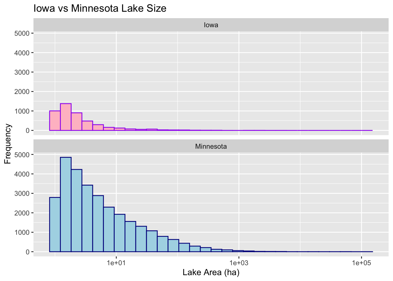

https://stackoverflow.com/questions/47596357/overlaying-two-ggplot-facet-wrap-histograms helped me write some of the histogram code chunk (for visualizations)

4.5 Interactive plot of lakes in Iowa and Illinois, colored them by lake area in hectares

#plotting iowa and illinois together
il_ia_lakes %>%
  arrange(-lake_area_ha) %>%
    slice(1:1000) %>%
  mapview(.,zcol = 'lake_area_ha')

4.6 Other data sources that I might use to understand how reservoirs and natural lakes vary in size in these three states?

Using data sets to quantify and gain a better understanding of lakes and reservoirs are very beneficial when looking at hydrological patterns, especially since climate change is looming over our heads. A journal from Michael Meyer, et. al, discusses how they combined different global datasets to create the most harmonic dataset that contains lake surface area, and water quantity and quality, and aquifer recharge at local, regional, and global scales. They combined, Global Water Bodies Data Base, LANDSAT data, and GRACE data to create this data set. This article shows how important it is to collect different types of data in order to create and discover the workings of our hydro-world. This large data set could help us understand the reservoirs and natural lakes in these states by showing us the recharge rates of the reservoirs.